Transform data for easier multi-column tables
gt
college basketball
cbbdata
tutorial
Creating 538-style captions with intuitive multi-column tables
The What
Dealing with multiple tables in gt is a pain, whether it be with gt_two_column_layout or some messy htmltools hacking. A clever way to address this is to transform your data into a wide format before you pass it to gt. This tutorial covers the latter and teaches you how to add what I’m calling a “538-style” caption (two captions separated by a black line at the bottom of the table).
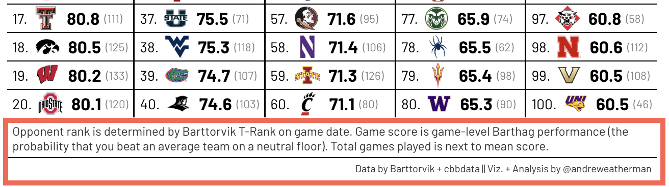
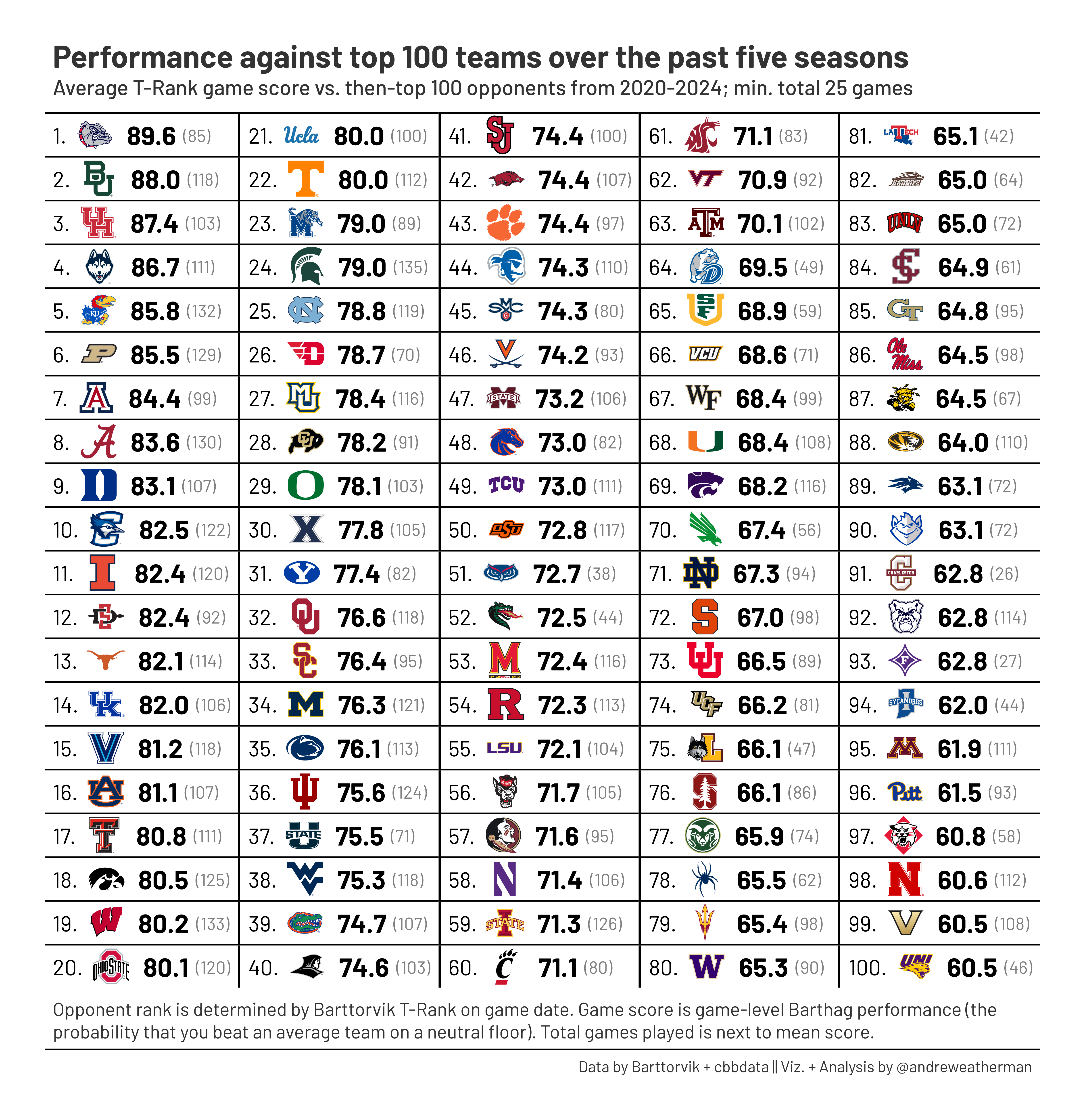
Using these ideas, we will be creating the table below – average team performance vs. top 100 opponents over the past five seasons in men’s college basketball.
The How
For this table, we will need:
The Data
Grabbing the data
For this visualization, we will be pulling data from Barttorvik using the cbbdata package.
data <- cbd_torvik_game_stats() %>%
  filter(year >= 2020) %>%
  left_join(cbd_torvik_ratings_archive() %>% select(opp = team, date, barthag, rank)) %>%
  filter(rank <= 100) %>%
  summarize(mean_score = mean(game_score),
            games = n(),
            .by = team) %>%
  filter(games >= 25) %>%
  slice_max(mean_score, n = 100) %>%
  arrange(desc(mean_score)) %>%
  left_join(cbd_teams() %>% select(team = common_team, logo))
Let’s break this down, we’re:
Pulling game-level data for every contest over the past five seasons
Appending the opponent’s Barttorvik rank entering the game
Filtering to include games vs. opponents inside the top 100
Averaging each team’s game score (you can think of this as game-level performance) and summing the number of contests played
Only considering teams who have played at least 25 games
Arranging by highest average score
Joining on team logos
| team | mean_score | games | logo |
|---|---|---|---|
| Gonzaga | 89.58000 | 85 | https://a.espncdn.com/i/teamlogos/ncaa/500/2250.png |
| Baylor | 87.97203 | 118 | http://a.espncdn.com/i/teamlogos/ncaa/500/239.png |
| Houston | 87.37087 | 103 | http://a.espncdn.com/i/teamlogos/ncaa/500/248.png |
| Connecticut | 86.74324 | 111 | http://a.espncdn.com/i/teamlogos/ncaa/500/41.png |
| Kansas | 85.83485 | 132 | http://a.espncdn.com/i/teamlogos/ncaa/500/2305.png |
| Purdue | 85.51163 | 129 | http://a.espncdn.com/i/teamlogos/ncaa/500/2509.png |
Creating an HTML column
Next, we’re going to create two important columns: group and formatted_score.
group is an indicator column on which we will split our data. For our table, we want to show the top 100 performing teams – and we’re going to do so with five 20-team columns. A simple way to indicate which team will be in which column is to create a new variable where teams 1-20 will be 1, teams 21-40 will be 2, and so on (any differentiation works). We can do this with rep(1:5, each = 20). The rep function will replicate the indicated set of values, in this case the sequence of [1, 2, 3, 4, 5], and the each parameter repeats each previous element 20 times. You can think of using the general form, rep(1:number_of_columns, each = total_rows_in_each_column).
formatted_score is an HTML column which will be rendered in using gt. Per usual, I’m not going to dive too deep into inline CSS or HTML. The basic functionality of this column is to show the team’s ranking, logo, average game score, and number of games played in a single cell. Our inline CSS forces the average game score to be bold and larger than the games text. The mean_score change simply rounds the average performance and formats it to show trailing zeros.
data <- data %>%
mutate(rank = row_number(),
group = rep(1:5, each = 20),
mean_score = round(mean_score, 1),
mean_score = ifelse(nchar(mean_score) == 2, glue("{mean_score}.0"), mean_score),
formatted_score = glue(
"<div style='display: flex; align-items: center;'>
{rank}.
<img src='{logo}' alt='Logo' style='height:25px; margin-right: 8px;'>
<span style='font-weight: bold; font-size: 1.2em; color: black; vertical-align: middle;'>{mean_score}</span>
<span style='font-size: 0.8em; color: gray; vertical-align: middle;'> ({games})</span>
</div>"
))Splitting our data
Now that we have our group and formatted_score column, we can pivot our data wider by splitting on our group number and binding the resulting lists together. The group_split function returns a list of tibbles that are separated by the associated group (i.e., the group number). The map_dfc function iterates over each list, selects columns containing “formatted_score,” and column-binds them into a single tibble – leaving us with a 20-row, 5-column data frame as intended.
The Table
Before we begin, a brief note: I’m in the process of developing a new package that will ship with a function to create the 538-style caption with a single line. For now, you’ll have to write the CSS yourself, or rather just copy mine, as there is no standalone function to do so.
The base
The base of our table uses the gt_theme_pl function from my cbbplotR package. The fmt_markdown function renders our HTML columns, cols_label removes all column labels, and cols_align center-aligns all columns. If you run this as-is and slap on a table header and caption, you’re honestly off to a pretty good start as the formatted_score columns and the gt_theme_pl function does much of the heavy lifting.
data %>%
  gt(id = "table") %>%
  gt_theme_pl() %>%
  fmt_markdown(contains("formatted_score")) %>%
  cols_label(everything() ~ "") %>%
  cols_align(columns = everything(), "center")
Adding dividers and adjusting fonts
To spice things up a bit, we will use gt_add_dividers to mimic row borders and the gt_set_font function from cbbplotR to choose a new table font. We can make our table a bit more compact by dropping the data_row.padding option to 1. By default, the table font in gt_theme_pl is a dark purple, and we can adjust this by setting our font color inside rows to black with tab_style and the cells_body location helper.
Note
In our gt_add_divider line, we did not select the final column because the function defaults to adding borders on the right side of the column, which would look funky on the last column.
... %>%
  gt_add_divider(columns = -last_col(), color = "black", weight = px(1.5), include_labels = FALSE) %>%
  gt_set_font("Barlow") %>%
  tab_options(data_row.padding = 1) %>%
  tab_style(locations = cells_body(), cell_text(color = "black"))
Annotations
You’re going to have to bear with me here. The way that I create the 538-style captions is by adding the top-level caption line, the one above the bottom border in the final table, as a footnote and later include some necessary CSS to make it work. Perhaps there is a way to do this by just using tab_source_note, and I bet there is, but I’m assuming that is a bit messier than my solution.
Importantly, if you do want this caption design, you’re going to have to sacrifice the ability to use table footnotes. You can easily write your footnote information in this top-level caption, but you won’t see the footnote marks.
... %>%
  tab_footnote(locations = cells_column_labels(), footnote = md("Opponent rank is determined by Barttorvik T-Rank on game date. Game score is game-level Barthag performance (the<br>probability that you beat an average team on a neutral floor). Total games played is next to mean score.")) %>%
  tab_header(
    title = "Performance against top 100 teams over the past five seasons",
    subtitle = "Average T-Rank game score vs. then-top 100 opponents from 2020-2024; min. total 25 games"
  ) %>%
  tab_source_note("Data by Barttorvik + cbbdata || Viz. + Analysis by @andreweatherman")
Necessary CSS
As promised, this table will rely on some CSS. I’m not really going to touch on anything but the footnote additions.
#table .gt_footnote adds a solid black line with width 1px below the table footnote, which we are treating as our top-level caption, and adjusts the font size. #table .gt_footnote_marks hides the footnote marks in the column headers as they are irrelevant in this design. #table .gt_sourcenote aligns our bottom-level caption, defined with tab_source_note, to the right of our table, mimicking the popular 538 table design.
... %>%
  opt_css(
    "
    #table .gt_column_spanner {
      border-bottom-style: none !important;
      display: none !important;
    }
    #table .gt_subtitle {
      line-height: 1.2;
      padding-top: 0px;
      padding-bottom: 0px;
    }
    #table .gt_footnote {
      border-bottom-style: solid;
      border-bottom-width: 1px;
      border-bottom-color: #000;
      font-size: 12px;
    }
    #table .gt_footnote_marks {
      display: none !important;
    }
    #table .gt_sourcenote {
      text-align: right;
    }
    #table .gt_row {
      border-top-color: black;
    }
    "
  )
Full Code
Data
data <- cbd_torvik_game_stats() %>%
filter(year >= 2020) %>%
left_join(cbd_torvik_ratings_archive() %>% select(opp = team, date, barthag, rank)) %>%
filter(rank <= 100) %>%
summarize(mean_score = mean(game_score),
games = n(),
.by = team) %>%
filter(games >= 25) %>%
slice_max(mean_score, n = 100) %>%
arrange(desc(mean_score)) %>%
left_join(cbd_teams() %>% select(team = common_team, logo)) %>%
mutate(rank = row_number(),
group = rep(1:5, each = 20),
mean_score = round(mean_score, 1),
mean_score = ifelse(nchar(mean_score) == 2, glue("{mean_score}.0"), mean_score),
formatted_score = glue(
"<div style='display: flex; align-items: center;'>
{rank}.
<img src='{logo}' alt='Logo' style='height:25px; margin-right: 8px;'>
<span style='font-weight: bold; font-size: 1.2em; color: black; vertical-align: middle;'>{mean_score}</span>
<span style='font-size: 0.8em; color: gray; vertical-align: middle;'> ({games})</span>
</div>"
)) %>%
group_split(group) %>%
map_dfc(~ select(.x, contains("formatted_score")))Table
table <- data %>%
  gt(id = "table") %>%
  gt_theme_pl() %>%
  fmt_markdown(contains("formatted_score")) %>%
  cols_label(everything() ~ "") %>%
  cols_align(columns = everything(), "center") %>%
  gt_add_divider(columns = -last_col(), color = "black", weight = px(1.5), include_labels = FALSE) %>%
  gt_set_font("Barlow") %>%
  tab_options(data_row.padding = 1) %>%
  tab_style(locations = cells_body(), cell_text(color = "black")) %>%
  tab_footnote(locations = cells_column_labels(), footnote = md("Opponent rank is determined by Barttorvik T-Rank on game date. Game score is game-level Barthag performance (the<br>probability that you beat an average team on a neutral floor). Total games played is next to mean score.")) %>%
  tab_header(
    title = "Performance against top 100 teams over the past five seasons",
    subtitle = "Average T-Rank game score vs. then-top 100 opponents from 2020-2024; min. total 25 games"
  ) %>%
  tab_source_note("Data by Barttorvik + cbbdata || Viz. + Analysis by @andreweatherman") %>%
  opt_css(
    "
    #table .gt_column_spanner {
      border-bottom-style: none !important;
      display: none !important;
    }
    #table .gt_subtitle {
      line-height: 1.2;
      padding-top: 0px;
      padding-bottom: 0px;
    }
    #table .gt_footnote {
      border-bottom-style: solid;
      border-bottom-width: 1px;
      border-bottom-color: #000;
      font-size: 12px;
    }
    #table .gt_footnote_marks {
      display: none !important;
    }
    #table .gt_sourcenote {
      text-align: right;
    }
    #table .gt_row {
      border-top-color: black;
    }
    "
  )
Saving the table
Per usual, I like to use my crop_gt function, also shipping with my upcoming package, to evenly trim whitespace included when using gtsave_extra.
crop_gt <- function(file, whitespace) {
  image_read(file) %>%
    image_trim() %>%
    image_border("white", glue('{whitespace}x{whitespace}')) %>%
    image_write(file)
}gtsave_extra(table, "performance_vs_top_100.png", zoom = 7)
crop_gt("performance_vs_top_100.png", 200)Parting Notes
As always, if you enjoy my work, I would greatly appreciate a share on Twitter. I’ll keep doing these tutorials as long as people find them helpful :)