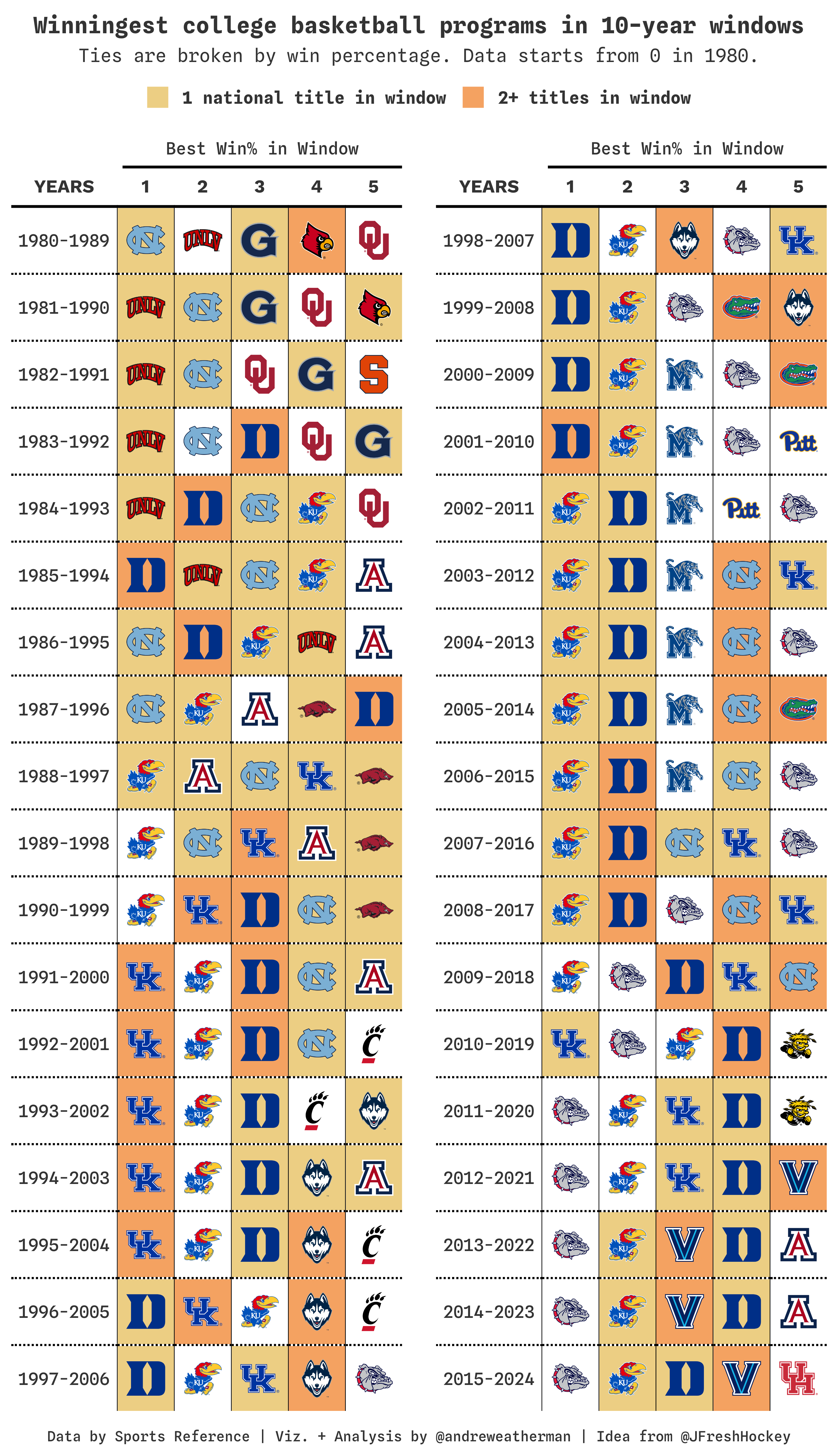
Total Wins in Rolling Windows
gt
college basketball
scraping
tutorial
Uh, a lot of
gt hacking…
Note
Fair warning: This code involves quite a bit of “hacking around.” Building HTML and CSS strings, adapting non-exported gtExtras functions, leveraging htmltools to splice everything together, etc. If anything, I hope some of my esoteric nonsense might prove useful in your own endeavors. If you’re a beginner, please look at some other gt tutorials as to not get discouraged! The package is wonderful and intuitive…except when it isn’t.
The What
In early May 2024, JFreshHockey posted a visualization showing the top five winningest teams in rolling ten-year windows in the NHL.
For our visualization, we will be looking at cumulative wins in rolling ten-year windows at the Division 1 level from 1980 to 2024. You can adapt this code to, instead, look at win percentage, losses, etc., at the national or conference level.
What we will be creating
The How
For this table, we will need:
The Data
Grab The Data
We need to grab per-season win totals from 1980 to 2024. There are a few ways to pull this data, but to keep things open and free, we will scrape individual season pages on Sports Reference and not use a paid source like Stathead.
We can grab season record by-year with rvest by iterating through https://www.sports-reference.com/cbb/seasons/men/{YEAR}-ratings.html. The data is stored in static tables, so a simple html_table function should do the trick here.
Using the SelectorGadget tool, we can find the tag associated with the standings table on every page.
Selector Gadget
Using a simple loop, we can grab per-season conference wins and losses. Here, we hit the ratings page, scrape the static table, “lift” it from the resulting list, and do some basic data manipulation.
janitor functions when scraping
If you’re relatively new to web scraping in R, take note of the row_to_names and clean_names functions (both from the janitor package). If the column names of your data are stored in some row in the returned frame, row_to_names will elevate that row to be the column names. You’ll routinely find that your column headers are stored in the first or second row when scraping Sports Reference.
clean_names “standardizes” your column names, which is sometimes just a nice touch and other times a necessity. Actually, if you remove that line from the function below, you’ll run into an error because the resulting tibble has a few columns with empty names. You won’t be able to do any mutate or filter. It’s recommended to run clean_names after row_to_names. (It’s my opinion that row_to_names should have an optional argument to do this without needing a separate call.)
season_results <- map_dfr(1980:2024, \(year) {
  Sys.sleep(3) # for 501 error

  suppressWarnings({
    read_html(glue("https://www.sports-reference.com/cbb/seasons/men/{year}-ratings.html")) %>%
      html_nodes("#ratings") %>% # target standings
      html_table() %>% # get table
      pluck(1) %>% # pluck from list
      row_to_names(1) %>% # first row are col. names
      clean_names() %>%
      mutate(year = year,
             across(w:l, as.numeric)) %>% # convert w and l to numeric
      filter(!is.na(w)) %>% # remove non-team rows
      select(team = school, wins = w, losses = l, year)
  })

}, .progress = 'Getting data')
This code will take around two to three minutes to run. Alternatively, you can download a copy of the data below.
Calculate the Windows
There are a few ways to apply a function, i.e. summing things, over a rolling window. zoo::rollapply is a nice method, and the slider package provides some useful functionality.
But, I’m going to do it a bit differently and write a function to loop over. I’m doing this because it’s, in my opinion, the most intuitive and accessible approach. All I’m using is basic dplyr functions.
This function takes a data frame and a starting year. It then filters between that starting year and nine years into the future, using between, to grab 10-year “windows.” For each team, denoted with .by inside summarize, it calculates total wins, total losses, and win percentage (we only need total wins, but I decided to grab more data in case you want to plot something else).
Easier grouping with
.by in dplyr
dplyr v1.1.0 brought per-operation grouping with .by/by. This released in early 2023, but for some reason, I still see a lot of people unnecessarily using group_by.
In several dplyr functions, including summarize, mutate, and filter, you can specify a grouping level that is only active within that verb – meaning there is no need to use group_by + ungroup!
There are some nuances to this, and you can read more about them here.
calculate_windows <- function(start_year, data) {
  data %>%
    filter(between(year, start_year, start_year + 9)) %>%
    summarize(
      total_wins = sum(wins),
      total_losses = sum(losses),
      win_percentage = total_wins / (total_wins + total_losses),
      seasons = n(),
      .by = team
    ) %>%
    mutate(years = paste(start_year, start_year + 9, sep="-"),
           begin = start_year,
           end = start_year + 9)
}
We can, again, use purrr to iterate over our function. We want to loop over the beginning of our sequence (1980) to the last observed year minus nine (2024 - 9 = 2015). This ensures that we capture the final complete window.
season_windows <- map_dfr(1980:2015, ~calculate_windows(.x, season_results))Finally, let’s choose the five winningest teams over each window. We are breaking ties by highest win percentage, so we need to specify desc(win_percentage) as our second argument inside arrange and then take the first five rows in each window.
plot_data <- season_windows %>%
  group_by(years) %>% # arrange does not support per-operation grouping
  arrange(desc(total_wins), desc(win_percentage), .by_group = TRUE) %>% # ignores grouping by default
  slice_head(n = 5) %>%
  mutate(position = row_number()) %>% # need position value for plotting
ungroup()| team | total_wins | total_losses | win_percentage | seasons | years | begin | end | position |
|---|---|---|---|---|---|---|---|---|
| North Carolina | 281 | 63 | 0.8168605 | 10 | 1980-1989 | 1980 | 1989 | 1 |
| Nevada-Las Vegas | 271 | 65 | 0.8065476 | 10 | 1980-1989 | 1980 | 1989 | 2 |
| Georgetown | 269 | 69 | 0.7958580 | 10 | 1980-1989 | 1980 | 1989 | 3 |
| Louisville | 250 | 96 | 0.7225434 | 10 | 1980-1989 | 1980 | 1989 | 4 |
| Oklahoma | 245 | 90 | 0.7313433 | 10 | 1980-1989 | 1980 | 1989 | 5 |
| Nevada-Las Vegas | 283 | 61 | 0.8226744 | 10 | 1981-1990 | 1981 | 1990 | 1 |
National titles
Below, we’re going to talk about how to fill gt cells based on some condition, and that will require us to pull national championship winners. For consistency, since this section is about “data,” I’ll just include that code here.
champs <- read_html('https://www.sports-reference.com/cbb/seasons/') %>%
  html_nodes("#seasons_NCAAM") %>%
  html_table() %>%
  pluck(1) %>%
  clean_names() %>%
  mutate(year = parse_number(tournament)) %>%
  select(year, team = ncaa_champion) %>%
  filter(year >= 1954 & year != 2020)
We are going to adapt the calculate_windows function from above to do the same thing with number of championships.
Let’s apply that in a similar fashion to calculate_windows. We’re also going to change the numeric counts of total_titles to a general categorical variable to assist in plotting.
Let’s join that information over to plot_data. Teams that are not present inside champs will show as NA. We will fill these with 0s.
| team | total_wins | total_losses | win_percentage | seasons | years | begin | end | position | total_titles |
|---|---|---|---|---|---|---|---|---|---|
| North Carolina | 281 | 63 | 0.8168605 | 10 | 1980-1989 | 1980 | 1989 | 1 | 1 |
| Nevada-Las Vegas | 271 | 65 | 0.8065476 | 10 | 1980-1989 | 1980 | 1989 | 2 | 0 |
| Georgetown | 269 | 69 | 0.7958580 | 10 | 1980-1989 | 1980 | 1989 | 3 | 1 |
| Louisville | 250 | 96 | 0.7225434 | 10 | 1980-1989 | 1980 | 1989 | 4 | 2+ |
| Oklahoma | 245 | 90 | 0.7313433 | 10 | 1980-1989 | 1980 | 1989 | 5 | 0 |
| Nevada-Las Vegas | 283 | 61 | 0.8226744 | 10 | 1981-1990 | 1981 | 1990 | 1 | 1 |
Getting Ready for Plotting
Everything before this point has been pretty straightforward. But uh, now it’s time to start the “hacking” that I promised at the start.
Conditional highlighting
Team Logos + Pivoting
In our table, we are going to highlight on three conditions: a) no national titles won inside the window, b) one national title won inside the window, and c) multiple national titles won inside the window. (We aren’t actually going to do anything with point A; we’ll just leave those cells as-is – “filled with white”).
But the problem is that conditional highlighting in gt is a bit weird because tab_style + cell_fill does not really work as one might expect. Namely, row and column vectors aren’t treated as separate pairs. If you pass through, e.g. rows = c(1, 2) and columns = c(5, 6) inside tab_style, you’ll fill four cells, not two, because tab_style doesn’t treat things as unique pairs.
Turns out, you can just build the CSS string for highlighting cells outside of the table and apply it directly with opt_css…but this is a bit convoluted when you are highlighting multiple things.
Okay, so how do we do that? First, let’s grab team logos by creating a named vector using cbd_logos from cbbdata. (cbbdata ships with a function to create a named vector for matching team names, and I’ll eventually do the same thing for logos.)
Okay, so we’re going to need to pivot our data, but if we do it now, things will work…but our resulting tibble loses a crucial piece of information: total_titles!
I thought of a nifty way to include that information without sacrificing the neatness of our pivoted table. We can create an HTML string using <img> tags to reference logo links and throw in an alt tag that refers to total_titles. Adding an alt tag is completely harmless in our static table.
Pivoting in
R
I’m not going to lie, pivoting was one of the few things that really took some time to “click.” I recommend looking over this vignette if you’re in the same boat.
plot_data <- plot_data %>%
  mutate(team = glue("<img src='{logos[team]}' alt={total_titles} style='height:30px; vertical-align:middle;'>")) %>%
  pivot_wider(id_cols = years, names_from = position, values_from = team)
Generating the CSS
The final part is to define a function that will generate our needed CSS. Our CSS needs to target an individual cell and set its background-color relative to the number of titles won in a window, which is included in our alt tag. We can use the base R functions arrayInd and which to return a matrix of row-column indices that point to where the specific alt tag is true.
We will then loop over these indices to generate a string in the structure of #table_id tbody tr:nth-child({row}) td:nth-child({column}) {{ background-color: {color}; }}.
This looping is done when generating the tables themselves, but the functions are defined below.
generate_css <- function(data, css_id, pattern, color) {
  indices <- arrayInd(
    which(str_detect(as.matrix(data), pattern)),
    .dim = dim(data)
  )
  map2_chr(
    .x = indices[, 1],
    .y = indices[, 2],
    .f = ~glue("#{css_id} tbody tr:nth-child({.x}) td:nth-child({.y}) {{ background-color: {color}; }}")
  )

}

patterns_colors <- tibble(
  pattern = c('alt=0', 'alt=1', 'alt=2+'),
  color = c('#ffffff', '#ECCE83', '#F4A261')
)
An example of the CSS rule for targeting specific instances with no national title:
[1] "#table tbody tr:nth-child(10) td:nth-child(2) { background-color: #ffffff; }"
[2] "#table tbody tr:nth-child(11) td:nth-child(2) { background-color: #ffffff; }"
[3] "#table tbody tr:nth-child(30) td:nth-child(2) { background-color: #ffffff; }"
[4] "#table tbody tr:nth-child(32) td:nth-child(2) { background-color: #ffffff; }"
[5] "#table tbody tr:nth-child(33) td:nth-child(2) { background-color: #ffffff; }"
Header + Legend
I went back and forth on how to style the table header. I thought about effectively removing the need for a legend by coloring specific text in the subtitle with the appropriate colors – ala 1 national title in window and 2+ titles in window – but I wanted to keep with the colored boxes theme of the body itself.
If you haven’t caught on by now, gt offers so much versatility because it effectively renders HTML, and you can do a lot of stuff with that. To build the legend boxes, we can create a span that uses inline-block with equal width and height (to make squares). We then “mush” everything together in a single <div>.
key_info <- tibble(
  color = c('#ECCE83', '#F4A261'),
  label = c("1 national title in window", '2+ titles in window')
)

key_html <- key_info %>%
  mutate(
    key_item = glue("<span style='display: inline-block; margin-right: 5px; width: 15px; height: 15px; background-color: {color};'></span><span style='margin-left: 5px;font-size:12px;vertical-align:20%'>{label}</span>")
  ) %>%
  pull(key_item) %>%
  paste(collapse = ' ')

full_header_html <- glue(
  "<div style='text-align: center;'>
    <div style='font-size: 16px; margin-bottom: 4px;'>Winningest college basketball programs in 10-year windows</div>
    <div style='font-size: 13px; margin-bottom: 10px;font-weight:normal'>Ties are broken by win percentage. Data starts from 0 in 1980.</div>
    <div>{key_html}</div>
  </div>"
)
Plotting
Building the table
The table itself is actually pretty simple. There isn’t much gt going here. Because we are building a two-column layout, we should define a function to build our table.
It’s important that we are slicing the right data for each “side” of the table, and the split line does exactly that. Next, we loop over the generate_css function that we created earlier, and we push the output into a single string with unlist and paste.
Finally, we build the table. Again, not too much going on here. The gt_theme_athletic function from cbbplotR does a lot of the styling for us. We use fmt_markdown to render our HTML strings, adjust the column headers, add column spanners, and render our title. Importantly, we need to add a placeholder for our table caption – more on that later. We add the conditional highlighting CSS with opt_css. We then loop over this table function to create a list of tables.
Warning
For two-column layouts with independent CSS rules, it’s vital that we define a table ID and pass that to our generate_css function. If you don’t do that, and summarily remove {#css_id} from the glue statement in the function itself, only one set of CSS rules will apply to both tables.
build_table <- function(data, split_level, css_id) {

  split <- if(split_level == 1) data %>% slice(1:(nrow(.) / 2)) else data %>% slice(floor(nrow(.) / 2) + 1:nrow(.))

  # map over patterns and colors to generate CSS
  css_rules <- map2(
    patterns_colors$pattern,
    patterns_colors$color,
    ~generate_css(split, css_id, .x, .y)
  )

  # combine all CSS rules into one string
  combined_css <- css_rules %>% unlist() %>% paste(collapse = "\n")

  table <- split %>%
    gt(id = css_id) %>%
    gt_theme_athletic() %>%
    fmt_markdown(-years) %>%
    tab_style(locations = cells_column_labels(), style = cell_text(weight = 'bold', size = px(13))) %>%
    tab_style(locations = cells_title("title"), style = cell_text(size = px(20))) %>%
    tab_spanner(columns = -years, label = "Best Win% in Window") %>%
    tab_header(html(full_header_html)) %>%
    tab_source_note("placeholder") %>%
    opt_css(combined_css)

  return(table)

}

# loop over to create two tables
tables <- list(build_table(plot_data, 1, 'first'), build_table(plot_data, 2, 'second'))
Putting the tables together
gtExtras ships with a convenient function to create a two-column layout, gt_two_column_layout, but this doesn’t work well with our HTML title – so we can’t use that. Doing some digging, I was able to recreate that effect in a way that works for us.
First, let’s handle another issue that arises when using gt_two_column_layout: table captions (source notes). The latter uses an unexported function from gtExtras to extract a table title + subtitle, its class, and its style to then pass through to htmltools when rendering the table.
I took that function and reworked it to do the same thing for source notes. Remember that placeholder caption? Well, the reason we included one was to access its styles.
extract_source_note <- function(table) {
  raw_html <- as_raw_html(table) %>%
    read_html()

  gt_source_note <- raw_html %>%
    xml_find_first("//*[contains(concat(' ',normalize-space(@class),' '),' gt_sourcenote ')]")

  gt_table_id <- raw_html %>%
    xml_find_all("//body/div") %>%
    xml_attr("id")

  s <- raw_html %>%
    xml_find_first("//style") %>%
    xml_contents() %>%
    xml_text() %>%
    gsub(gt_table_id, "mycombinedtable", x = .) %>%
    gsub("mycombinedtable table", "mycombinedtable div", x = .)

  list(
    source_note = gtExtras:::xml_missing(gt_source_note),
    source_note_class = paste("gt_table", xml_attr(gt_source_note, "class")),
    source_note_style = xml_attr(gt_source_note, "style"),
    style = s
  )
}
Now, let’s apply the gtExtras function and the one above to extract our annotations (title, subtitle, and caption). Since both tables’ information is analogous, we only need to apply these functions to one table.
header_data <- gtExtras:::extract_tab_header_and_style(tables[[1]])
caption_data <- extract_source_note(tables[[1]])
Finally, we can use the htmltools package to generate an HTML container (div) that includes our tables and annotations! You can think of this as building the output vertically, where the title + subtitle go first, then the tables, and then our caption.
For the tables, we need to remove the individual annotations. Conveniently, you can set tab_header(NULL, NULL) to remove the title and subtitle, but for the caption, just setting tab_source_note(NULL) won’t actually work. You need to use the rm_source_notes function.
double_tables <- htmltools::div(
  id = "mycombinedtable", # need this exact ID
  ## table
  htmltools::tag("style", header_data[["style"]]),
  htmltools::div(
    htmltools::HTML(full_header_html),  # Your custom header HTML
    class = header_data[["title_class"]],
    style = header_data[["title_style"]]
  ),
  htmltools::div(tables[[1]] %>% gt::tab_header(NULL, NULL) %>% rm_source_notes(), style = "display: inline-block;float:left;"),
  htmltools::div(tables[[2]] %>% gt::tab_header(NULL, NULL) %>% rm_source_notes(), style = "display: inline-block;float:right;"),
  ## caption
  htmltools::tag("style", caption_data[["style"]]),
  htmltools::div(
    "Data by Sports Reference | Viz. + Analysis by @andreweatherman | Idea from @JFreshHockey",  # Your custom header HTML
    class = caption_data[["source_note_class"]],
    style = caption_data[["source_note_style"]]
  )
)
To view the output.
htmltools::browsable(double_tables)To save the output.
gtsave_extra(double_tables, "wins_since_1980.png", vwidth = 595, vheight = 1500, zoom = 5)